Slide 1 of 26
Slide 1 - Probability Theory and Random Variables
Probability Theory and Random Variables
Fundamentals, Distributions, and Applications
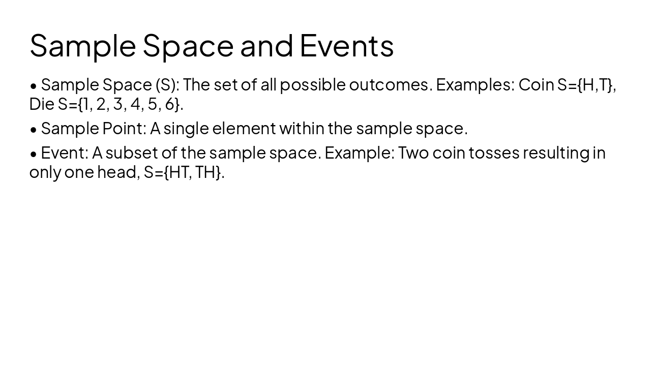
---
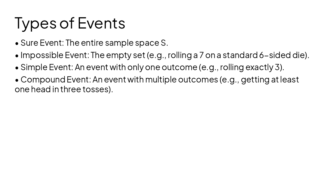
Photo by Deng Xiang on Unsplash
Generated from prompt:
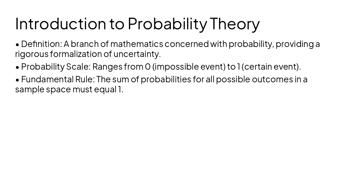
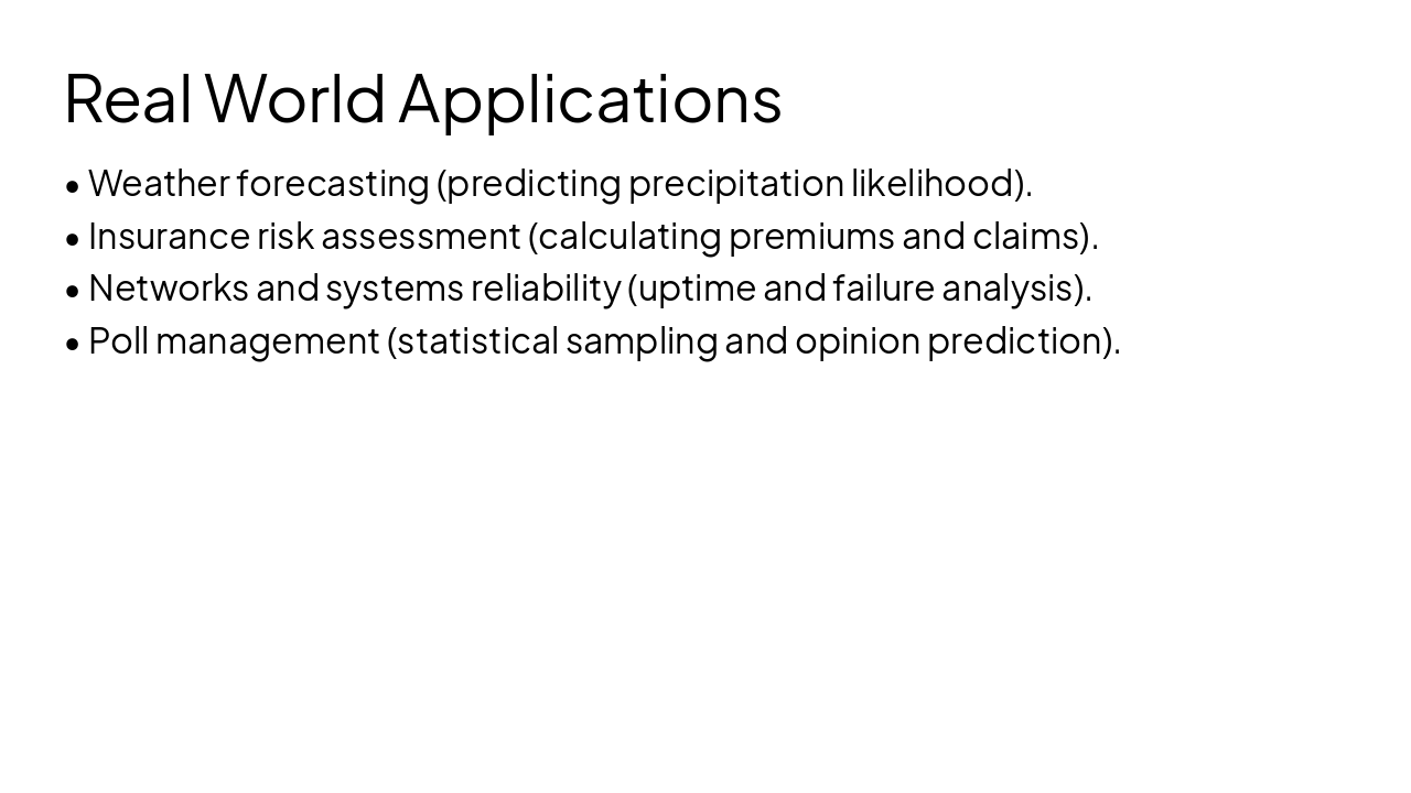
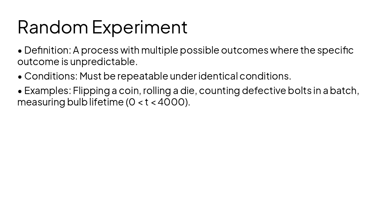
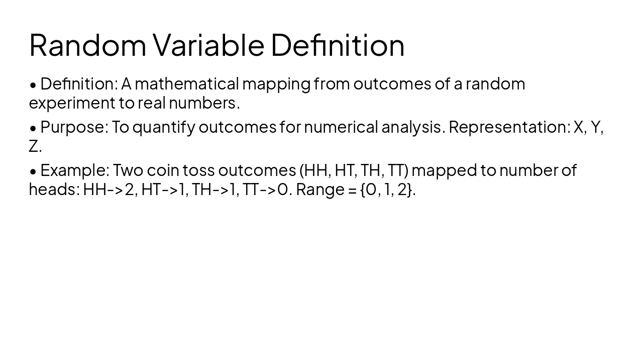
Create a PowerPoint presentation titled 'Probability Theory and Random Variables'. Use the provided slide structure exactly and do not remove any content. Slides: 1 Introduction to Probability Theory with definition, probability scale (0 impossible,1 certain), rule sum=1. 2 Real World Applications: weather forecasting, insurance risk, networks/systems reliability, poll management. 3 Random Experiment definition, conditions (multiple outcomes, unpredictable), examples coin/die, defective bolts, bulb lifetime 0<t<4000. 4 Sample Space and Events with examples coin S={H,T}, die S={1..6}, sample point, event subset example two coins only one head. 5 Types of Events: sure event S, impossible event empty set example rolling 7, simple event example exactly 3 on die, compound event at least one head in three tosses. 6 Bayes Theorem (heading only). 7 Random Variable definition, purpose, representation X,Y,Z; example two coin toss mapping HH->2 HT->1 TH->1 TT->0 range {0,1,2}. 8 Mapping S to R with X:S→R; examples die mapping and two coins mapping to number of heads. 9 Examples of Random Variables: heads in 3 tosses, customers per hour, bulb lifespan, defective items among 10. 10 Discrete Random Variable definition, countable values, examples students in class, telephone calls, number of heads; mention binomial and poisson. 11 Continuous Random Variable definition, examples height, weight, temperature, race time; mention uniform and normal distributions. 12 Range of Random Variable with examples two coins {0,1,2} and sum of two dice {2..12}. 13 Probability Distribution Function for continuous variable with properties non‑negative, total area 1, probability as area; formula P(a≤X≤b)=∫ab f(x)dx. 14 Cumulative Distribution Function F(x)=P(X≤x) properties 0–1, non‑decreasing, limit→1; relation to PDF via integration. 15 Binomial Distribution criteria n trials, success p failure q=1-p independence; formula P(X=k)=C(n,k)p^k q^{n-k}. 16 Binomial example defective bolts n=4 p=0.10 find P(X=1)=4*(0.1)*(0.9)^3=0.2916 conclusion 29.16%. 17 Poisson (heading only). 18 Uniform Distribution definition f(x)=1/(b-a) for a≤x≤b and probability formula integral equals (x2-x1)/(b-a); examples bus waiting time 0–10 min and random point on 1m ruler. 19 Mean and Variance of Uniform μ=(a+b)/2 variance (b-a)^2/12 explanation midpoint and interval length. 20 Problems Uniform: X uniform -2 to 6 mean=2 variance=64/12; P(X<4)=6/8; P(X>0)=6/8=3/4. Problem2 uniform 8–20 mean14 variance12; P(|X−6|≤15)=1; P(15≤X≤17)=1/6. 21 Normal/Gaussian Distribution definition with pdf (1/(σ√(2π)))e^{-(x-μ)^2/(2σ^2)}, bell shaped symmetric; examples heights IQ measurement errors. 22 Standard Normal Distribution Z=(X-μ)/σ Z~N(0,1) pdf φ(z)=(1/√(2π))e^{-z^2/2} purpose universal table. 23 Area Under Normal Curve properties total area1; P(μ−σ<X<μ+σ)=0.6826 explanation using Z. 24 Standard Normal Table how to use steps and examples Z=1.00 area0.3413 Z=1.96 area≈0.4750. 25 Comparison Uniform vs Normal example uniform(8,20) P(15≤X≤17)=1/6≈0.1667 vs normal μ=14 σ²=12 giving ≈0.1937 conclusion different shapes different probabilities. Design: academic clean theme, clear headings, math formatted, include simple diagrams where relevant (bell curve, uniform line).
Comprehensive introduction to probability theory, covering random experiments, sample spaces, events, discrete and continuous random variables, key distributions (Binomial, Poisson, Uniform, Normal), Bayes' Theorem, and real-world applications like天气
Probability Theory and Random Variables
Fundamentals, Distributions, and Applications
---
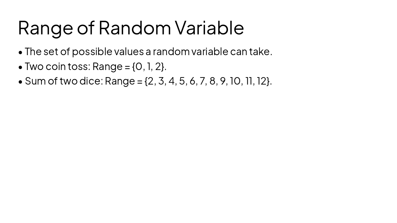
Photo by Deng Xiang on Unsplash
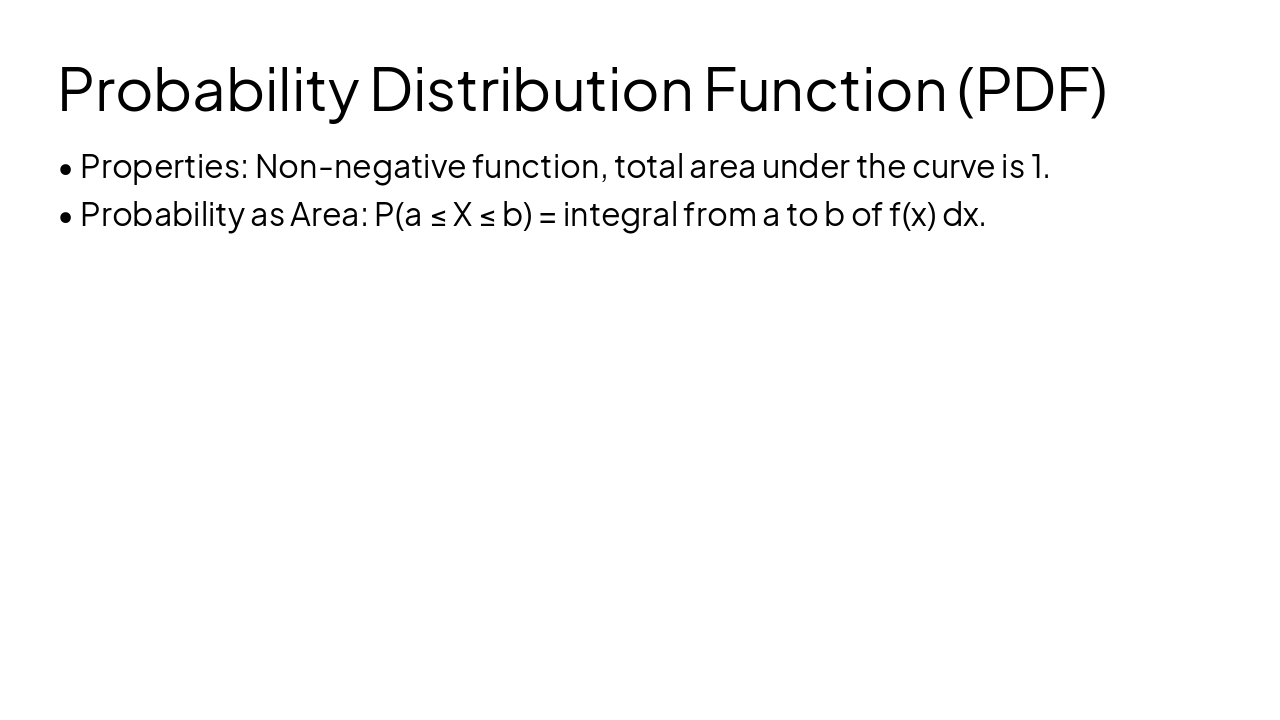
Advanced Conditional Probability
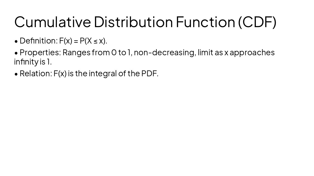
---
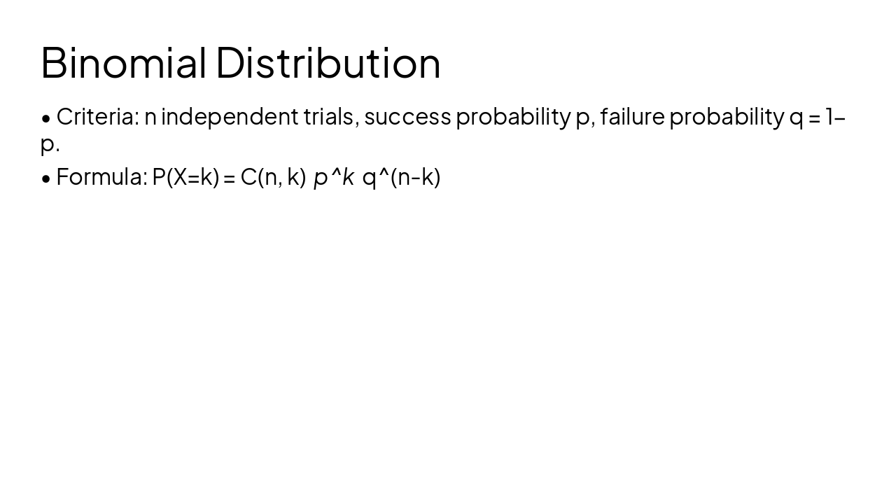
Photo by Shubham Dhage on Unsplash
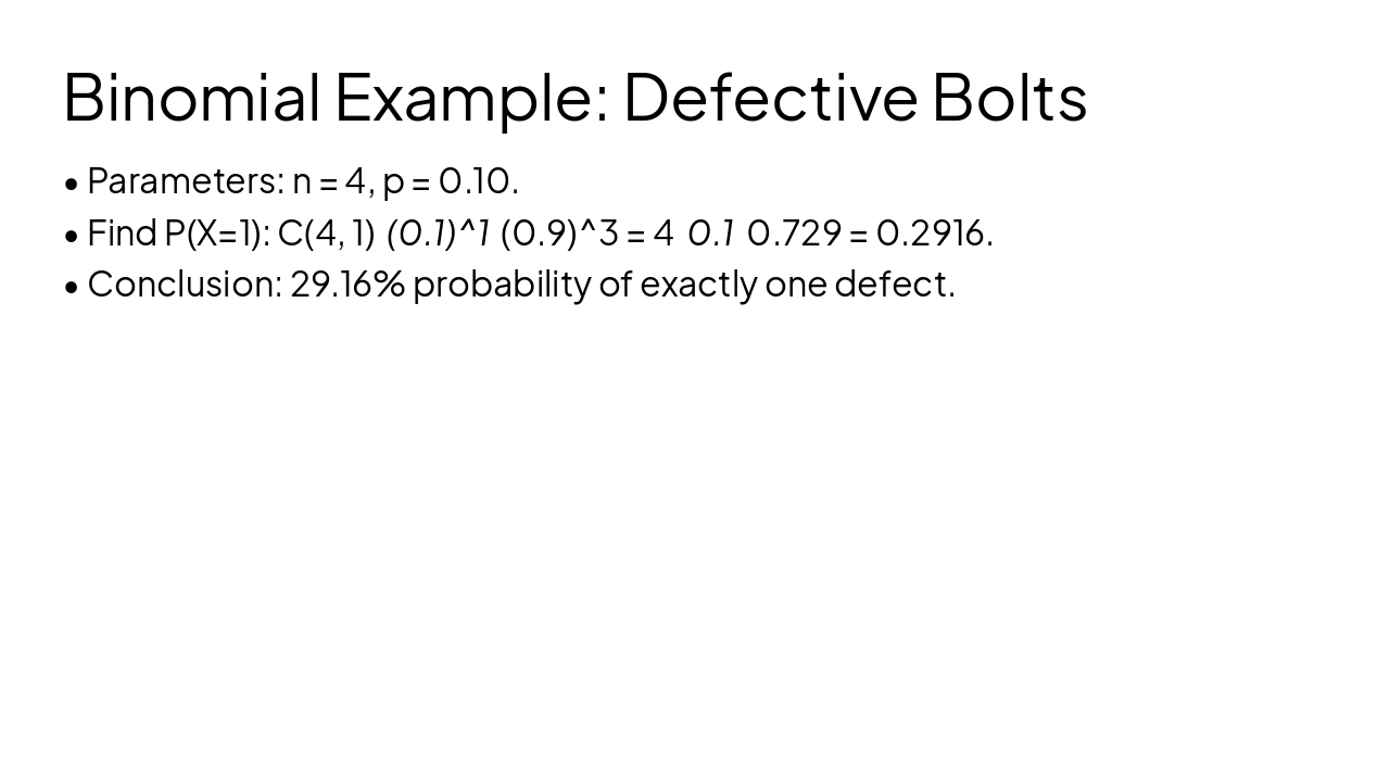
Modeling rare events in fixed intervals
---
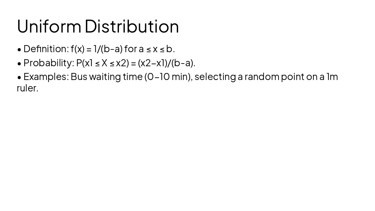
Photo by Deng Xiang (https://unsplash.com/@dengxiangs?utmsource=karaf&utmmedium=referral) on Unsplash (https://unsplash.com/?utmsource=karaf&utmmedium=referral)

Explore thousands of AI-generated presentations for inspiration
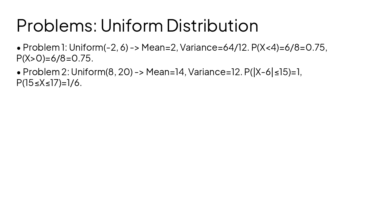
Generate professional presentations in seconds with Karaf's AI. Customize this presentation or start from scratch.